
Chapters:
1: Introduction
2: Simple example
3: Invocation
4: Finer Control
5: X-Y Plots
6: Contour Plots
7: Image Plots
8: Examples
9: Gri Commands
10: Programming
11: Environment
12: Emacs Mode
13: History
14: Installation
15: Gri Bugs
16: Test Suite
17: Gri in Press
18: Acknowledgments
19: License
Indices:
Concepts
Commands
Variables
5: X-Y Plots
- Linegraphs: x-y graphs with data connected by line segments
- Scattergraphs: x-y graphs with data indicated by symbols
- Formula Plots:
5.1: Linegraphs
The following Gri commands will draw a linegraph. For the output graph (see Getting More Control).This plots a simple linegraph:
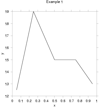
# Example 1 -- Linegraph using data in a separate file |
Here's what the command lines mean:
-
The first line is a comment. Anything to the right of a hash-mark
`
#' is considered to be a comment. (This symbol is also called a "pound".) - The second line is blank. Gri ignores blank lines between commands.
-
`
open example1.dat' tells Gri to open the indicated file (in the current directory) as an input data file. You can specify files outside the current directory by using conventional unix-shell pathnames (e.g., `open ~/data/TS/section1/T_S.dat' or `open ../data/file.dat'). You can even use "synonyms" (see Synonyms.) in filenames, as in `open \BASENAME.dat'. -
`
read columns x y' tells Gri to start reading columnar data, the first column being `x', the second `y'. `x' and `y' are predefined names for whatever ends up on the horizontal and vertical axes.The number of data needn't be specified. Gri reads columns until a blank line or end-of-file is found. You can tell Gri how many lines to read with a command like `
read columns 10 x y'. Multiple datasets can reside within one file; provided that they are separated by a single blank line, Gri can access them by multiple `read' commands.Like C, Gri expects numbers to be separated by one or more spaces or tabs. Commas are not allowed. If the columns were reversed, the command would be `
read columns y x'. If there were an initial column of extraneous data, the command would be `read columns * x y', or `read columns x=2 y=3' (see Read Columns). -
`
draw curve' tells Gri to draw a curve connecting the points in the `x' and `y' columns. A nice scale will be selected automatically. (You can change this or any other plot characteristics easily, as you'll see later.) -
`
draw title' tells Gri to write the indicated string centered above the plot. The title must be enclosed in quotes. -
`
quit' tells Gri to exit.
Gri will draw axes automatically, and pick its own scales.
If you wish to draw several curves which cross each other, you should
try using `draw curve overlying' instead of
`draw curve'. This will make it easier to distinguish the
different curves.
5.2: Scattergraphs
This section contains two examples, the first being a fuller explanation of all the bells and whistles, the second being a simple explanation of how to get a very quick plot, given just a file containing a matrix of grid data.
To get a scattergraph with symbols at the data points, substitute
`draw symbol' for `draw curve'. Both symbols and a curve
result if both `draw curve' and `draw symbols' are used.
See see Getting More Control for an example.
By default, the symbol used is an x. To get another symbol, use a
command like `draw symbol 0' or `draw symbol plus'.
To change the symbol size from the default of 0.2 cm use commands like
`set symbol size 0.1' to set to 1 mm (see Set Symbol Size).
5.2.1: Coding data with symbols
To get different symbols for different data points, insert symbol codes from the above list as a column along with the x-y data, and substitute the command `read columns x y z', and then draw them with
`draw symbol'. Gri will interpret the rounded-integer
values of the `z' columns as symbol codes. Note that even if
you've read in a z column which you intend to represent symbols, it will
be overridden if you designate a specific symbol in your
`draw symbols' command; thus `draw symbol 0' puts a `+'
at the data points whether or not you've read in a symbol column.
5.2.2: Drawing a symbol legend
The following example shows how you might write a symbol legend for a plot. The legend is drawn 1 cm to the right of the right-hand side of the axes, with the bottom of the legend one quarter of the way up the plot; see Draw Symbol Legend. The lines in the legend are double-spaced vertically. To change the location of the legend, alter the `.legend_x. =' and `.legend_y. =' lines. To change the
spacing, alter the `.legend_y. +=' line.
set x axis -1 5 1 set y axis -1 5 1 read columns x y z 0 0 0 1 1 1 2 2 2 3 3 3 |
5.2.3: Coding data with symbol colors
To get different colors for different symbols, read a color code into the z column, and do for example `draw symbol bullet color hue z'.
The numerical color code ranges from 0 (red) through to 1, passing
through green at 1/3 and blue at 2/3.
5.3: Formula Plots
There are two methods for formula graphs.
- Use the system yourself.
Do as in this example:
open "awk 'BEGIN{for(i=0;i<3.141;i+=0.05)\ {print(i,cos(i))}}' |" read columns x y close draw curve - Let Gri calculate things for you
The simplest is to let Gri calculate things for you with the `
create columns from function' command (see Create). The command assumes that you have defined the synonym called `\function' which defines `y' in terms of `x'.Gri uses the program `
awk' to create the columns, and cannot work without it.Here is an example of using `
create columns from function':show "First 2 terms of perturbation expansion" set y axis name horizontal set y name "sea-level" set x name "$\omega$t"
\b = "0.4" # perturbation parameter b=dH/H \xmin = "0" \xmax = "6.28" \xinc = "3.14 / 20" \function = "cos(x)" set x axis \xmin \xmax create columns from function draw curve draw title "SOLID LINE \function"
\function = "(cos(x)+\b/2*(1-cos(2*x)))" create columns from function set dash 1 draw curve draw title "DASHED LINE \function"
draw title "b = \b"
Here's another example, in which the curve `
y = 1/(\int + \sl*x)' is drawn through some data. Note how `sprintf' is used to set `\xmin' and `\xmax' using the scales that Gri has determined in reading the data.open file.data read columns x y close draw symbol bullet \int = "-0.1235" \sl = "0.003685" sprintf \xmin "%f" ..xleft.. sprintf \xmax "%f" ..xright.. \function = "1/(\int + x * \sl)" create columns from function draw curve
