9.3.9: The `draw' commands

NOTE Gri likes drawings to have axes, so if a `draw' command is executed before any axes have been drawn, Gri will draw axes after it draws the item. (You can get drawings without axes by preceding any other `draw' commands with the command `draw axes none'.) Many users have been surprised by the results of this rule. For example, if you do `set graylevel 0.5' before `draw curve', you'll find that the axes are drawn in gray also. To avoid this, make sure to do `draw axes' before you modify the graylevel.)

• Draw Arc: Draw an arc segment
• Draw Arrow: Draw single arrow
• Draw Arrows: Draw many arrows (using columns)
• Draw Axes If Needed: Draw axes if haven't done so yet
• Draw Axes: Draw axes
• Draw Border Box: Draw border around plot
• Draw Box: Draw a box, possibly filled
• Draw Circle: Draw a circle
• Draw Contour: Draw contour(s)
• Draw Curve: Draw a curve of y(x) column data
• Draw Essay: Draw text, adjusting position for each line
• Draw Gri Logo: Draw a Gri logo
• Draw Grid: Draw the location of grid points
• Draw Image Histogram: Draw histogram of values in image
• Draw Image Palette: Draw palette used in image plots
• Draw Image: Draw image
• Draw Isopycnal: Draw isopycnal line on TS plot
• Draw Isospice: Draw iso-spice line on TS plot
• Draw Label Boxed: Draw a label in a box
• Draw Label Whiteunder: Draw a label with white ink under it
• Draw Label For Last Curve: What it says
• Draw Label: Draw text somewhere
• Draw Line From: Draw line segment
• Draw Line Legend: Draw legend displaying line types
• Draw Lines: Draw sequence of parallel lines
• Draw Patches: Draw grayscale patches showing z(x,y)
• Draw Polygon: Draw a polygon
• Draw Regression Line: Draw line from regression between x and y
• Draw Symbol At: Draw a symbol at a point
• Draw Symbol Legend: Draw a symbol and a string describing it
• Draw Symbol: Draw symbols at (x,y), or at a point
• Draw Time Stamp: Draw a timestamp at top of plot
• Draw Title: Draw a title for plot
• Draw Values: Draw numbers beside z(x,y)
• Draw X Axis: Draw the x axis
• Draw X Box Plot: Draw box plots showing x spread
• Draw Y Axis: Draw the y axis
• Draw Y Box Plot: Draw box plots showing y spread
• Draw Zero Line: Draw y=0 or x=0

9.3.9.1: The `draw arc' command

`draw arc [filled] .xc_cm. .yc_cm. .r_cm. .angle_1. .angle_2.'

Draw an "arc", that is, a portion of a circle. The center of the circle is at the coordinate (`.xc_cm.', `.yc_cm.'), and the circle radius is `.r_cm.', all three quantities being in cm on the page, not in user-units. The arc starts at angle `.angle_1.', measured in degrees counterclockwise from a horizontal line, and extends to angle `.angle_2.', in the same units.

If the keyword `filled' is present, the arc is filled with the current color. Otherwise it is drawn with the current "curve" linewidth see Set Line Width.

9.3.9.2: `draw arrow'

draw arrow from .x0. .y0. to .x1. .y1. [cm]

With no optional parameters, draw an arrow from (`.x0.', `.y0.') to (`.x1.', `.y1.'), where coordinates are in user units. The arrow head will be at (`.x1.', `.y1.'), and its size is as set by most recent call to `set arrow size'. With the `cm' keyword present, the coordinates are in centimetres on the page. NOTE: This will not cause auto-drawing of axes.

9.3.9.3: `draw arrows'

`draw arrows'

Draw a vector field consisting of arrows emanating from the coordinates stored in the (x, y) columns. The lengths and orientations of the arrows are stored in the (u, v) columns, and the scale for the (u,v) columns is set by `set u scale' and `set v scale'. See also (1) To set arrow size, use `set arrow size'. (2) To get a single arrow, use `draw arrow'.

9.3.9.4: `draw axes if needed'

`draw axes if needed'

Draw axes frame if required. Used within gri commands that auto-draw axes. NOTE: this should only be done by developers.

9.3.9.5: `draw axes'

`draw axes [.style.|frame|none]'

With no style (`.style.') specified, draw x-y axes frame labelled at left and bottom. The value of `.style.' determines the style of axes:

• `.style. = 0' Draw x-y axes frame labelled at left and bottom. Since this is the default, it's best to leave it out altogether to make your code easier to understand.

• `.style. = 1' Draw axes without tics at top and right

• `.style. = 2' Draw axes frame with no tics or labels; same as `draw axes frame'

With the keyword `frame' specified, draw axes frame with no tics or labels (just like `.style.' = 2, but preferable because it makes for code that is easier to read and understand).

With the keyword `none' specified, prevent Gri from automatically drawing axes when drawing curves.

Note: `set axes style' can also be used to set axes properties, and then simply using `draw axes', or letting axes be auto-drawn, will result in the desired effect (see Set Axes Style). However, if the `draw axes' command explicitly asks for a particular style, then it over-rides the style set by `Set Axes Style'.

9.3.9.6: `draw border box'

`draw border box .xleft. .ybottom. .xright. .ytop. \
    .width_cm. .brightness.'

Draw gray box, as decoration or alignment key for pastup. The box, with outer lower left corner at (`.xleft.', `.ybottom.') and outer upper right corner at (`.xright'., `.ytop.') -- both coordinates being in centimetres on the page -- is drawn with thickness `.width_cm.' and with graylevel `.brightness.' (0 for black; 1 for white). The gray line is drawn inside the box. After drawing the gray line, a thin black line is drawn along the outside edge.

If the geometry is not specified with `.xleft.' and the other parameters, then a reasonable margin is used around the present axes area, and the defaults (`.border.' = 0.2, `.brightness.' = 0.75) are used.

NOTE: This command does not cause auto-drawing of axes.

9.3.9.7: `draw box'

`draw box filled .xleft. .ybottom. .xright. .ytop. [cm|pt]'

Draw filled box spanning indicated range, with lower-left corner at (`.xleft.', `.ybottom.') and upper-right corner at (`.xright.', `.ytop.'). The corners are specified in user coordinates, unless the optional `cm' or `pt' keyword is present, in which case they are in centimetres or points on the page. An error will result if you specify user coordinates but they aren't defined yet.

No checking is done on the rectangle; for example, there is no requirement that `.xleft.' be to the left of `.xright.' in your coordinate system.

NOTE: if the box is specified in user units, this command will cause auto-drawing of axes, but not if the box is specified in `cm' or `pt' units

`draw box .xleft. .ybottom. .xright. .ytop. [cm|pt]'

Draw box spanning indicated range, with lower-left corner at (`.xleft.', `.ybottom.)' and upper-right corner at (`.xright.', `.ytop.').

The corners are specified in user coordinates, unless the optional `cm' or `pt' keyword is present, in which case they are in centimetres or points on the page. An error will result if you specify user coordinates but they aren't defined yet.

No checking is done on the rectangle; for example, there is no requirement that `.xleft.' be to the left of `.xright.' in your coordinate system.

9.3.9.8: `draw circle'

draw circle with radius .r_cm. at .x_cm. .y_cm.

Draw circle of specified radius (in cm) at the specified location (in cm on the page).

9.3.9.9: `draw contour'

`draw contour [{.value. \
  [unlabelled | {labelled "\label"}]} \
  | {.min. .max. .inc. \
    [.inc_unlabelled.] [unlabelled]}]'

This command draws contours based on the "grid" data previously read in by a `read grid data' command or created by gridding column data with a `create grid from columns' command. If the grid data don't exist, or if the x and y locations of the grid points do not exist (see `set x grid', `set y grid', etc), Gri will complain.

With no optional parameters, draw labelled contours at an interval that is picked automatically based on the range of the data. With a single numerical value (`.value.'), draw the indicated contour. With the addition of `labelled "\label"', put the indicated label instead of a numeric label. This can be useful for using scientific notation instead of computer notation for exponents, e.g. `draw contour 1e-5 labelled "10$^{-5}$"'.

With (`.min.', `.max.' and `.inc.') given, draw contours for z(x,y) = `.min.', z(x,y) = `.min. + .inc.', z(x,y) = `.min. + 2*.inc.', ..., z(x,y) = `.max.'

With the additional value `.inc_unlabelled.' specified, extra unlabelled contours are drawn at this finer interval.

With the optional parameter `unlabelled' at the end of any form of this command (except the `labelled "\label"' variation, of course), Gri will not label the contour(s).

Hint: It can be effective to draw contours at a certain interval with labels, and a thicker pen, e.g.

set line width rapidograph 3x0 draw contour -2 5 1 0.25 set line width rapidograph 1 draw contour -2 5 1

Interpolation method: The interpolation scheme is the same used for converting grid-values to image values (see Convert Grid To Image).

See also `set contour labels'

9.3.9.10: `draw curve'

`draw curve'

Draws a curve connecting the points (x,y), which have been read in by a command like `read columns x y'. Line segments are drawn between all (x,y) points, except: (1) no line segments are drawn to any missing data (see `set missing value'), and (2) if clipping is turned on (see `set clip on'), no line segments are drawn outside the clipping region. See also `draw curve overlying'

`draw curve overlying'

Like `draw curve', except that before drawing, the area underneath the curve (+/- one linewidth) is whited out. This clarifies graphs where curves overlie other curves or the axes. See also `draw curve'.

`draw curve filled [to {.y. y}|{.x. x}]'

The form `draw curve filled ...' draws filled curves. If the `to .value.' is not specified, fill the region defined by the x-y points using the current paint colour (see `set graylevel'). To complete the shape, an extra line is drawn between the first and last points.

The form `draw curve filled to .y. y' fills the region between y(x) and y = `.y.'; do not connect the first and last points as in the case where `to .yvalue.' is not specified.

The form `draw curve filled to .x. x' fills the region between x(y) and x = `.x.'

9.3.9.11: `draw essay'

`draw essay "text"|reset'

Draw indicated text on the page. Succeeding calls draw text further and further down the page, starting at the top.

The current font size is used; to alter this, use `set font size' before `draw essay'.

When `reset' is present instead of text, the drawing position is reset to the top of the page. Use this after a `new page' command to ensure that the next text lines will appear at the top of the page as expected. EXAMPLE:

set font size 2 cm draw essay "Line 1, at top of page" draw essay "Line 2, below top line"

9.3.9.12: `draw gri logo'

`draw gri logo .x_cm. .y_cm. .height_cm. .style. \fgcolor \bgcolor'

Draw a Gri logo at given location with given style and colors. The lower-left corner of the logo will be `.x_cm.' centimeters from the left-hand side of the page and `.y_cm.' centimeters from the bottom of the page. The logo will be `.height_cm.' centimeters tall. The textual parameters `\fgcolor' and `\bgcolor' give the foreground and background colors, respectively, and these are used in styles as noted in the table below

.style. style ======= =================== 0 stroke curve 1 fill with color \fgcolor, no background 2 fill with color \fgcolor it in tight box of color \bgcolor 3 as 2 but in square box 4 draw in \fgcolor on top of shifted copy in \bgcolor

An example is given below

draw gri logo 1 1 3 4 blue green

9.3.9.13: `draw grid'

`draw grid'

Draw plus-signs at locations where grid data are non-missing.

9.3.9.14: `draw image histogram'

`draw image histogram \
  [box .llx_cm. .lly_cm. .urx_cm. .ury_cm.]'

With no optional parameters, draw histogram of all unmasked parts of the image, placing it above the current top of the plot.

When the `box' options are present, they specify the box (in centimetre coordinates on the page) in which the histogram plot is to be done.

9.3.9.15: `draw image palette'

`draw image palette 
   [axisleft|axisright|axistop|axisbottom] 
   [left .left. right .right. [increment .inc.]] 
   [box .xleft_cm. .ybottom_cm. .xright_cm. .ytop_cm.]'

With no optional parameters, draw palette for image, placed above the current top showing values ranging from `.min_value.' to `.max_value.' as given in `set image range'.

Optional keywords (`axisleft', etc) control the orientation of the palette, the default being `axisbottom'.

The optional parameters `.left.' and `.right.' may be used to specify the range to be drawn in the palette. If the additional optional parameter `.inc.' is present, it specifies the interval between tics on the scale; if not present, the tics are at increments of 2 * (`.right.' - `.left'.). (If `.inc.' has the wrong sign, it will be corrected without warning.)

When the optional `box' parameters are present, they prescribe the bounding box to contain the palette. The units are centimetres on the page. If these parameters are not present, the box will be drawn above the image plot.

Hint It is a good idea to make the palette range `.left.' to `.right.' extend a little beyond the range of full white and full black, since otherwise neither pure white nor pure black will appear in the colorbar. For example

set image grayscale black 0 white 1 increment 0.1 draw image palette left -0.1 right 1.1 increment 0.1

Hint Continuous-tone images with superimposed contours are often effective. To get the contour lines drawn on the image palette, do something like this

draw image .left. = 0 .right. = 9 .inc. = 1 .space. = 3 .height. = 1 draw image palette left .left. \ right .right. \ increment .inc. \ box \ ..xmargin.. \ {rpn ..ymargin.. ..ysize.. + .space. + } \ {rpn ..xmargin.. ..xsize.. +} \ {rpn ..ymargin.. ..ysize.. + .space. + .height. + } draw contour .left. .right. .inc. unlabelled .c. = .left. while {rpn .right. .c. <= } .c_cm. = {rpn .c. .left. - \ .right. .left. - / \ ..xsize.. * ..xmargin.. +} draw line from \ .c_cm. \ {rpn ..ymargin.. ..ysize.. + .space. + }\ to \ .c_cm. \ {rpn ..ymargin.. ..ysize.. + .space. + .height. +} \ cm .c. += 1 end while

9.3.9.16: `draw image'

`draw image'

Draw black/white image made by `convert grid to image' or by `read image'.

9.3.9.17: `draw isopycnal'

`draw isopycnal \
   [unlabelled] .density. [.P_sigma. [.P_theta.]]'

Draw isopycnal curve for a temperature-salinity diagram. This curve is the locus of temperature and salinity values which yield seawater of the indicated density, at the indicated pressure. The UNESCO equation of state is used.

For the results to make sense, the x-axis should be salinity and the y-axis should be either in-situ temperature or potential temperature.

The `.density.' unit is kg/m^3. If the supplied value exceeds 100 then it will be taken to indicate the actual density; otherwise it will be taken to indicate density minus 1000 kg/m^3. (The deciding value of 100 kg/m^3 was chosen since water never has this density; the more intuitive value of 1000 kg/m^3 would be inappropriate since water can have that density at some temperatures.) Thus, 1020 and 20 each correspond to an actual density of 1020 kg/m^3.

The reference pressure for density, `.P_sigma.', is in decibars (roughly corresponding to meters of water depth). If no value is supplied, a pressure of 0 dbar (i.e. atmospheric pressure) is used.

The reference pressure for theta, `.P_theta.', is in decibars, and defaults to zero (i.e. atmospheric pressure) if not supplied. This option is used if the y-axis is potential temperature referenced to a pressure other than the surface. Normally the potential temperature is, however, referenced to the surface, so that specifying a value for `.P_theta.' is uncommon.

By default, labels will be drawn on the isopycnal curve; this may be prevented by supplying the keyword `unlabelled'. If labels are drawn, they will be of order 1000, or of order 10 to 30, according to the value of `.density.' supplied (see above). The label format defaults to "%g" in the C-language format notation, and may be controlled by `set contour format'. The label position may be controlled by `set contour label position' command (bug: only non-centered style works). Setting label position is useful if labels collide with data points. Labels are drawn in the whiteunder mode, so they can white-out data below. For this reason it is common to draw data points after drawing isopycnals.

If the y-axis is in-situ temperature, the command should be called without specifying `.P_sigma.', or, equivalently, with `.P_sigma.' = 0. That is, the resultant curve will correspond to the (S,T) solution to the equation

.density. = RHO(S, T, 0)

where `RHO=RHO(S,T,p)' is the UNESCO equation of state for seawater. This is a curve of constant sigma_T.

If the y-axis is potential temperature referenced to the surface, `.P_theta.' should not be specified, or should be specified to be zero. The resultant curve corresponds to a constant value of potential density referenced to pressure `.P_sigma.', i.e. the (S,theta) solution to the equation

.density. = RHO(S, theta, .P_sigma.)

For example, with `.P_sigma.=0' (the default), the result is a curve of constant sigma_theta.

If the y-axis is potential temperature referenced to some pressure other than that at the surface, `.P_theta.' should be supplied. The resultant curve will be the (S,theta) solution to the equation

.density. = RHO(S, T', .P_sigma.)

where

T'=THETA(S, theta, .P_theta., .P_sigma.)

where `THETA=THETA(S,T,P,Pref)' is the UNESCO formula for potential temperature of a water-parcel moved to a reference pressure of `Pref'. Note that `theta', potential temperature referenced to pressure `.P_theta.', is the variable assumed to exist on the y-axis.

9.3.9.18: `draw isospice'

`draw isospice .spice. [unlabelled]'

Draw an iso-spice line for a "TS" diagram, using (S, T) data stored in files in a subdirectory named `iso-spice0' in a directory named by the unix environment variable `GRI_EOS_DIR'. You must set this environment variable yourself, in the normal unix way. If `GRI_EOS_DIR' is not defined, Gri looks in the directory `/data/po/ocean/EOS/iso0'; of course, this will work only for people on the same machine as the author.

Only certain iso-spice lines are stored in these files, so only certain values of `.spice.' are allowed. They are 21.75, 22.00, 22.25, ..., 30.75. You must supply `.density.' in exactly this format (with 2 decimal places), or else Gri will not find the appropriate TS file, and will give a "can't open file" error. NB: isopycnals ranging from about 23.00 to 26.00 cross a TS diagram spanning 34<S<36 and 0<T<10.

The line is labelled at the right with the density value, unless the `unlabelled' option is given.

Clipping should be on when drawing iso-spice lines. A warning will be given if the isospice line does not intersect the clipping region.

EXAMPLE

set clip on draw isospice line 27.00 draw isospice line 27.50 unlabelled

9.3.9.19: `draw label'

`draw label boxed "string" at .xleft. .ybottom. [cm]'

Draw boxed label for plot, located with lower-left corner at indicated (x,y) position (specified in user units or in cm on the page). The current font size and pen color are used. The geometry derives from the current font size, with the label being centered within the box.

9.3.9.20: `draw label whiteunder'

`draw label whiteunder "\string" at .xleft. .ybottom. [cm]'

Draw label for plot, located with lower-left corner at indicated (x,y) position (specified in user units or in cm on the page). Whiteout is used to clean up the area under the label. BUGS: Cannot handle angled text; doesn't check for super/subscripts.

9.3.9.21: `draw label for last curve'

`draw label for last curve "label"'

Draw a label for the last curve drawn, using the `..xlast..' and `..ylast..' built-in variables.

9.3.9.22: `draw label'

`draw label "\string" [centered|rightjustified] \
    at .x. .y. [cm|pt] \
    [rotated .deg.]'

With no optional parameters, draw string at given location in USER units.

With the `cm' or `pt' keyword is present, the location is in centimetres or points on the page.

With the `rotated' keyword present, the angle in degrees from the horizontal, measured positive in the counterclockwise direction, is given.

With the keyword `centered' present, the text is centered at the given location; similarly the keyword `rightjustified' makes the text end at the given location.

9.3.9.23: `draw line from ... to'

`draw line from .x0. .y0. to .x1. .y1. [cm|pt]'

With no optional parameters, draw a line from (`.x0.', `.y0.') to (`.x1.', `.y1'.), where coordinates are in user units. With the `cm' or `pt' keyword present, the coordinates are in centimetres or points on the page. NOTE: This will not cause auto-drawing of axes.

9.3.9.24: `draw line legend'

`draw line legend "label" at .x. .y. [cm] [length .cm.]'

Draw a legend identifying the current line type with the given label. A short horizontal line is drawn starting at the location (`.x.', `.y.'), which may be specified in centimetres or, the default, in user coordinates. The line length is normally 1 cm, but this length can be set by the last option. The indicated label string is drawn 0.25 cm to the right of the line. See also `draw symbol legend ...'. EXAMPLE (of keeping track of the desired location for the legend)

.offset. = 1 # cm to offset legends # ... get salinity data set line width 0.25 draw curve draw line legend "Salinity" at .x. .y. # ... get temperature data set line width 1.0 set dash 0.45 0.05 draw curve .y. += .offset. draw line legend "Temperature" at .x. .y.

9.3.9.25: `draw lines'

`draw lines {vertically .left. .right. .inc.} | \
    {horizontally .bottom. .top. .inc.}'

Draw several lines, either vertically or horizontally. This can be useful in drawing gridlines for axes, etc. The following example shows how to draw thin gray lines extending from the labelled tics on the x axis (ie, at 0, 0.1, 0.2, ... 1):

set x axis 0 1 0.1 0.05 set y axis 10 20 10 draw axes set graylevel 0.75 set line width 0.5 draw lines vertically 0 1 0.1 set graylevel 0

9.3.9.26: `draw patches'

`draw patches .width. .height. [cm]'

With the optional `cm' keyword not present, draw column data z(x,y) as gray patches according to the grayscale as set by most recent `set image grayscale'. The patches are aligned along the horizontal, and have the indicated size in user units.

With the optional keyword `cm' is present, the patch size is specified in centimetres.

9.3.9.27: `draw polygon'

`draw polygon [filled] .x0. .y0. .x1. .y1. [...]'

Draw a polygon connecting the indicated points, specified in user units. The last point is joined to the first by a line segment. At least two points must be specified. If the `filled' keyword is present, the polygon is filled with the current pen color.

9.3.9.28: `draw regression line'

`draw regression line [clipped]'

Fit and draw a regression line to column data, of the form `y = ..coeff0.. + ..coeff1.. * x', exporting `..coeff0..', `..coeff0_sig..', `..coeff1..' and `..coeff1_sig..' as global variables (see Regress).

Normally, the line is not clipped to the axes frame, but it will be if the keyword `clipped' is given.

HINT: to label the plot you might do the following:

sprintf \label "y = %f + %f * x. R$^2$=%f" \ ..coeff0.. ..coeff1.. ..R2.. draw title "The linear fit is \label"

9.3.9.29: `draw symbol ... at'

`draw symbol .code.|\name at .x. .y. [cm|pt]'

Draw a symbol at given (single) location. The location is normally in user coordinates; it will be in centimetres on the page if the optional `cm' or `pt' keyword is given.

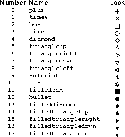
With the optional numerical/name code specified, then the symbol of that number or name is drawn at each (x,y) datum, whether or not a z-column exists. The numerical/name codes are:

9.3.9.30: `draw symbol legend'

`draw symbol legend \symbol_name "label" \
    at .x. .y. [cm]'

Draw indicated symbol at indicated location, with the indicated label beside it. The label is drawn one M-space to the right of the symbol, vertically centered on the indicated `.y.' location.

9.3.9.31: `draw symbol'

`draw symbol [[.code.|\name]    \
    | [graylevel z]             \
      [color [hue z|.h.]        \
             [brightness .b.]   \
             [saturation .s.]]]'

With no optional parameters, draw symbols at the (x,y) data. If a z-column has been read with `read columns', then its value codes the symbol to draw, according to the table below. (The value of z is first rounded to the nearest integer.) If no z-column has been read, the symbol X is drawn at each datum.

With the optional numerical/name code specified, then the symbol of that number or name is drawn at each (x,y) datum, whether or not a z-column exists. The numerical/name codes are:

With the optional `graylevel z' fields specified, the graylevel is given by the `z' column (0=black, 1=white).

With the optional `color' field specified, the color is specified, either directly in the command (the `hue .h.' form) or in the z column. For more information on color, refer to the `set color hsb ...' command.

Examples: both `draw symbol bullet color' and `draw symbol bullet color hue z' draw bullets whose hue is given by the value in the z column. The hue (or the color, in other words) blends smoothly across the spectrum as the numerical value ranges from 0 to 1. The value 0yields red, 1/3 yields green, 2/3 yields blue, etc. If the `brightness' and the `saturation' are not specified, they both default to the value 1, which yields pure, bright colors.

Example: draw all in green dots `draw symbol bullet color hue 0.333 brightness 1 saturation 1'

Example: display spectrum of dots

set symbol size 0.3 open "awk 'END{ \ for(c=0;c<1;c+=1/40) \ print(c,c,c)}' | " read columns x y z close draw symbol bullet color hue z

9.3.9.32: `draw time stamp'

`draw time stamp \
    [fontsize .points. \
        [at .x_cm. .y_cm. cm \
            [with angle .deg.]]]'

Draw the command-file name, PostScript file name, and time, at the top of graph. Normally, the timestamp is drawn at the top of the page, in a fontsize of 10 points. But the user can specify the fontsize, and additionally the location (in cm) and additionally the angle measured in degrees anticlockwise from the horizontal.

NOTE: If you want to have the plot drawn in landscape mode, ensure that `set page landscape' precedes `draw time stamp.'

9.3.9.33: `draw title'

`draw title "\string"'

Draw the indicated string above the plot.

9.3.9.34: `draw values'

draw values                 \
    [.dx. .dy.]             \
    [\format]               \
    [separation .xcm. .ycm.]

Draw values of `z' column, at corresponding (`x', `y') locations. If the `separation' keyword is present, the distance between successive points is checked, and points are skipped unless the x and y separations exceed the indicated distances.

• `draw values' Draw the values of `z(x,y)', positioned 1/2 M-space to the right of `(x,y)' and vertically centred on `y'. The values are written in a good general format known as `%lg', in C terminology.

• `draw values %.2f' Draw values of `z(x,y)' positioned as described above, but using the indicated format string. This format string specifies that 2 numbers be used after the decimal place, and that floating point should be used. See any C manual for format codes.

• `draw values .dx. .dy.' Print values of `z(x,y)' at indicated offset vector (`.dx.',`.dy.'), measured in centimeters, from the values of `(x,y)' at which the data are defined.

• `draw values .dx. .dy. %.3f' Print values of `z(x,y)' at indicated distance from `(x,y)', indicated format.

9.3.9.35: `draw x axis'

draw x axis [at bottom|top|{.y. [cm]} [lower|upper]]

Draw an x axis, optionally at a specified location and of a specified style.

• `draw x axis' Draw a lower x axis (ie, one with the numbers below the line) at the bottom of the box defined by `set y axis'.

• `draw x axis at bottom' Draw a lower x axis (ie, one with the numbers below the line) at the bottom of the box defined by `set y axis'.

• `draw x axis at top' Draw an upper x axis (ie, one with the numbers above the line) at the top of the box defined by `set y axis' (or above any existing stacked x axes there)

• `draw x axis at .y.' Draw a lower x axis at indicated value of `.y.'.

• `draw x axis at .y. upper' Draw an upper x axis at indicated value of .y.

9.3.9.36: `draw x box plot'

draw x box plot at .y. [size .cm.]

Draw Tukey box plots (which give a summary of histogram properties). Box plots were invented by Tukey for eda (exploratory data analysis). The centre of the box is the median. The box edges show the first quartile (q1) and the third quartile (q3). The distance from q3 to q1 is called the inter-quartile range. The whiskers (i.e., the lines with crosses at the end) extend from q1 and q3 to the furthest data points which are still within a distance of 1.5 inter-quartile ranges from q1 and q3. Beyond the whiskers, all outliers are shown: open circles are used for data within a distance of 3 inter-quartile ranges beyond q1 and q3, and in closed circles beyond that.

• `draw x box plot at .y.' Draw Tukey's box plot, spreading in the x direction, centered at y=`.y.' and of default width 0.5 cm.

• `draw x box plot at .y. size .cm.' Draw Tukey's box plot, spreading in the x direction, centered at y=`.y.' and of width `.cm.' centimetres.

9.3.9.37: `draw y axis'

draw y axis [at left|right|{.x. cm} [left|right]]

Draw a y axis, optionally at a specified location and of a specified style.

• `draw y axis' Draw a left-hand-side y axis (ie, one with the numbers to the left of the line) at left of box defined by `set x axis'

• `draw y axis at left' Draw a left-hand-side y axis (ie, one with the numbers to the left of the line) at left of box defined by `set x axis'.

• `draw y axis at right' Draw a right-hand-side y axis (ie, one with the numbers to the right of the line) at right of box defined by `set x axis'.

• `draw y axis at .x.' Draw a left-hand-side y axis (ie, one with the numbers to the left of the line) at indicated value of `.x.'

• `draw y axis at .x. right' Draw a right-hand-side y axis (ie, one with the numbers to the right of the line) at indicated value of `.x.'

9.3.9.38: `draw y box plot'

draw y box plot at .x. [size .cm]

Draw Tukey box plots (which give summary of histogram properties).

• `draw y box plot at .x.' Draw Tukey's box plot, spreading in the y direction, centered at x=`.x.' and of default width 0.5 cm.

• `draw y box plot at .x. size .cm.' Draw Tukey's box plot, spreading in the y direction, centered at x=`.x.' and of width `.cm.' centimetres.

9.3.9.39: `draw zero line'

draw zero line [horizontally|vertically]

Draw lines corresponding to x=0 or y=0.

• `draw zero line' Draw line y=0 if it is within axes.

• `draw zero line horizontally' Draw line y=0 if it is within axes.

• `draw zero line vertically' Draw line x=0 if it is within axes.