
Chapters:
1: Introduction
2: Simple example
3: Invocation
4: Finer Control
5: X-Y Plots
6: Contour Plots
7: Image Plots
8: Examples
9: Gri Commands
10: Programming
11: Environment
12: Emacs Mode
13: History
14: Installation
15: Gri Bugs
16: Test Suite
17: Gri in Press
18: Acknowledgments
19: License
Indices:
Concepts
Commands
Variables
6: Contour Plots
Contour plots can be done with either pregridded data or randomly distributed (ie, ungridded) data.- Pre-gridded Data: Contouring f(x1, y1, x2, y2, ...)
- Ungridded Data: Contouring f(x, y) where (x,y) are not on a grid
6.1: Pre-gridded Data
This section presents two examples of contouring pre-gridded data, the first example illustrating a boilerplate program to contour data stored in a simple matrix form in a file, the second example illustrating a case with more control of the details (e.g., a nonuniform grid).
6.1.1: Simple example
This example was hardwired to know the size of the grid, etc. Here's an example which is more general, in that it determines the dimensions of the grid data from using unix system commands. Note that the grid is set to run from 0 to 1 in both x and y; you'll most likely want to change that after you see the initial plot, but this should get you started.
\file = "somefile.dat"
\rows = system wc \file      | awk '{print $1}'
\cols = system head -1 \file | awk '{print NF}'
set x grid 0 1 /\cols
set y grid 0 1 /\rows
open \file
read grid data \rows \cols
close
draw contour
|
6.1.2: Complicated example
To get a simple contour graph based on pre-gridded data, with full control of axes, etc, do something like this:
Here several new things have been introduced.
First, you've got to define a grid in xy space. This example uses a
non-uniform x-grid, and reads it in from the commandfile. In this form,
the blank line is essential; it tells Gri that the end of data has been
located; if you like, you can specify the number of lines to read, as in
`read grid x 3'.
The y-grid for this example is uniform, however, so it may be specified
with the `set y grid' command. It obtains values (10, 12.5, 15,
17.5, 20). The `set x|y grid' commands accept negative increments.
Furthermore, it is possible to specify the number of steps, rather than
the increment size, by putting `/' before the third number; thus
`set x grid 0 1 /5' and `set x grid 0 1 0.2' are equivalent.
Having defined a grid, it is time to read in the gridded data. Here this
is done with the `read grid data' command. Since Gri already knows
the grid dimensions, it will read the data appropriately. You could
also have told it (`read grid data 3 5').
The first dataline is the top of the y-grid. In other words, the data appear in the file just as they would on the graph, assuming that the x-grid and y-grid both increase.
Sometimes you want to read in the transpose of a matrix. Gri lets you
do that. If the `bycolumns' keyword is present at the end of the
`read grid' command, the first dataline will contain the first
column, of the data.
If you have an extraneous column of data to the left of your data
matrix, do `read grid data * 2 3'
Now Gri has the grid in its head. We tell it to draw some contours
with the `draw contour' command. As the comments in the example
show, the contour values will be selected automatically, but you can
alter that.
6.2: Ungridded data
When you have f=f(x,y) points at random x and y, you must cast them onto a grid to contour them. This is a difficult problem. There are many ways to grid data, and all have both good and bad features. You should try various methods, and various settings of the parameters of the methods. If you have a favorite gridding method that you prefer, you should probably pre-grid the data yourself. If not, Gri can do it for you. Gri has two methods for doing this, the ``boxcar'' method and the ``objective analysis'' method. Each method puts holes in the grid wherever there are too few data to map to grid points, unless you specifically ask to fill in the whole grid.The next two sections show first an example, then a discussion of the methods and how to use them.
6.2.1: Example
This example uses data taken from Figure 5 of S. E. Koch and M. DesJardins and P. J. Kocin, 1983. ``An interactive Barnes objective map anlaysis scheme for use with satellite and conventional data,'', J. Climate Appl. Met., vol 22, p. 1487-1503. Readers should compare Figures 5 and 6 of that paper to the results shown here.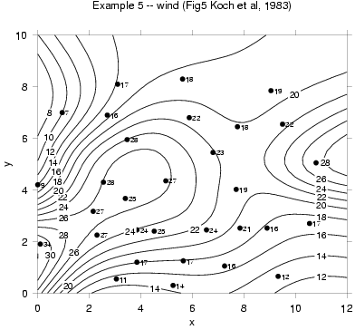
6.2.2: Discussion of Methods
The various commands for converting columns to a grid are given in (see Convert Columns To Grid). Generally, the Barnes method is best.
